02 · Mixture of Experts

Committee or Competition

Two ways to combine several networks, and only one of them specialises.

The previous topic explained one architecture of interest which is a layer that holds a great deal of parameters and uses only a few of them on any given token. That wish is about compute, and it is how mixtures of experts are usually motivated today.

The interference problem

Nowlan and Hinton open with the difficulty in one sentence: if backpropagation is used to train a single network to perform different subtasks on different occasions, there will generally be strong interference effects which lead to slow learning and poor generalisation. Every weight is pulled by every case. Cases that need different behaviour pull in different directions, and what settles is a compromise that suits neither.

The proposal introduces a collection of distinct sub-networks, defined as the experts , alongside a dedicated routing module known as the gating network . The sole responsibility of the gate is to analyze the current input and assign it to the appropriate expert.

The term "gating" here can be misleading, as it suggests a simple on/off switch when it is actually nothing of the sort. The gate is an ordinary neural network, usually a small multi-layer perceptron that takes the input, passes it through zero or more hidden layers, and ends in an output layer with exactly one unit per expert. In the original experiments, the gate sometimes had five or ten hidden units, and sometimes none at all, making it a single linear layer and nothing more.

The values sitting at those output units, before any normalisation, are the scores . There is one score per expert, and is the network's raw, unbounded opinion about how suitable expert is for this input. Being unbounded, the scores are not yet a routing decision given that they can be negative, they can be large, and they do not sum to anything in particular.

Concretely, in the simplest case where the gate has no hidden layers, producing the scores is a single matrix multiplication:

is the input the gate is shown, of size .
is the gate's weight matrix, with one row per expert. Row is a direction in input space, and is how far the input points along it.
is the bias, one per expert.

A gate with several hidden layers

Number the layers and let . Each hidden layer is

and the output layer, which produces the scores, is

with , where is the width of layer . Only two of those widths are forced: , the size of the input, and , one output unit per expert. Everything in between is a free choice. The single-layer case above is .

The layer index is written in parentheses, , because a bare superscript already means the training case, as in . And the hidden nonlinearity is written rather than , because is the width of the Gaussians further down this page.

With hidden layers this is the last of several such steps, and nothing about the argument changes. What matters is that and are learned, by the same gradient descent that trains the experts. Nobody writes down a routing rule. The gate discovers one, and later on this page we derive exactly what the gradient arriving at turns out to be.

The case's input enters a small multi-layer perceptron whose output layer has one unit per expert. The four pre-softmax values 1.2, minus 0.4, 2.7 and 0.1 are the scores. A softmax turns them into gate values of 0.17, 0.03, 0.74 and 0.06, which weight the four experts, and the arrow into the third expert is much thicker than the others.

The gate is a network like any other. What makes it a gate is the shape of its output layer, one unit per expert.

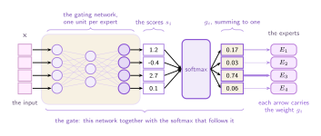
To turn the scores into a routing decision we need them non-negative and summing to one, so they can be read as probabilities. That is exactly what the softmax function does:

The exponential makes every value positive and the denominator makes them sum to one, so the largest score becomes the largest share without any of them ever reaching zero. From the first paper onwards the are read as the probability of selecting expert .

One piece of notation before we go further. A case is one training example which contains an input together with a target we want the network to predict. When we need to tell one case from another we write it as a superscript, so and are the input and the target of case , and is what the gate said about expert on that case. A sum written runs over the training set and a sum written runs over the experts. The figure below illustrates this process.

At the top, one input runs through the gate to three scores of plus 0.4, plus 2.1 and minus 0.6, and a softmax turns them into a bar of height one split into 0.15, 0.80 and 0.05. Below, a table with one row per case and one column per expert holds the gate's outputs, with a brace across the first row showing that it sums to one and a brace under the second column showing that it sums to 1.44 down the training set. — The two indices do different work. Across a row the gate splits one case between the experts, so the row sums to one. Down a column it accumulates how much of the training set an expert was handed, and that quantity is the one every load argument later in the series is about.

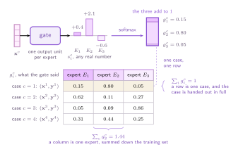
Here a case is a whole training example, because that is what these networks were built to handle: one input, one target, one decision by the gate. From Compute You Can Skip onwards a case is a single token inside a sequence, and the gate makes its decision several times per example rather than once.

Two ways to combine them

Defining a multi-network architecture with a gate does not yet tell us how this mechanism should learn. Let's go through this learning process.

The committee

The standard ensemble approach is to blend the outputs via the gate and compute the error on the final prediction. Let represent the individual output vector produced by the -th expert. The overall network prediction is given as a weighted sum of these expert outputs proportioned by the gate's activation . That is,

Look at what it does to an individual expert. The error is computed after the blend, so an expert receives gradient signals based on the committee's collective performance rather than their own. The expert is told whether the committee was right, and it is nudged by its share of that. If expert 2 is already good on this case and expert 1 is badly wrong, the loss still pulls expert 1 toward the same target, because the global loss cannot disentangle individual contributions, it merely treats Expert 1's output as a deficit in the aggregate prediction. Thus, every expert is trained to reduce the residual of the others. Under a squared error on the blend, the best thing any expert can do is learn the average of everything, which is the interference we were trying to escape.

The competition

The alternative is to measure each expert on its own, and blend the measurements rather than the outputs. Treat each expert as predicting the mean of a Gaussian, treat the gate as supplying the mixing proportions, and take the negative log probability of the target under that mixture:

is the error on training case .
is the gate's output for expert on the case .
is the desired output and the output of expert .
is a constant, the width of each Gaussian.

The outputs are vectors, as they are in the original paper. Since is a single shared width, each expert defines a spherical Gaussian centred on its own prediction, and is the distance from the target to that centre. Everything below holds unchanged for a one-dimensional output, where the norm is read as an absolute value.

The two expressions might look similar, but their behavior is fundamentally changed by swapping the order of operations. Instead of blending the predictions, this equation treats each expert's output as the center of its own Gaussian distribution. The inner term directly measures how well Expert alone explains the target. The gate then scales this by the expert's assigned routing probability.

By summing these independent probabilities before applying the logarithm, the loss evaluates the mixture as a whole without forcing the experts' outputs to average out. If even a single expert perfectly hits the target, the sum inside the logarithm becomes large, the overall loss drops, and the other experts are left alone rather than being dragged in to compensate. The figure below illustrates the process for each combination strategy.

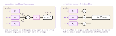
Two panels. On the left, three experts feed a weighted sum, the sum is compared with the target, and gradient arrows of equal thickness return to all three experts. On the right, each expert is compared with the target on its own, the three likelihoods are combined inside a logarithm, and the gradient arrow returning to the middle expert is far thicker than the other two.

Blending before the measurement makes the experts cooperate. Measuring before the blend makes them compete, and the arrows coming back are the whole difference.

It's important to highlight the gradient effect of the architectures above. The committee takes a weighted sum of outputs and then measures the error. The competition measures the error of each expert separately, takes a weighted sum of those probabilities, and then applies the logarithm. But why does this matter? Because the summation happens inside the logarithm which allows the gradients to decouple. If one expert is highly accurate, it dominates the sum, minimizing the loss for that specific case. The remaining experts aren't penalized or forced to adjust their weights to fix a residual gap. They are simply ignored for that case. This is somewhat a "true competition" in the sense that experts are rewarded for individual specialization, not for collective compromise, allowing each one of them to specialize.

Prior, posterior, and the gradient between them

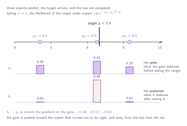
The competition reading gives us a second quantity that the committee formulation does not have, before the target arrives, the gate's output is a prior, meaning it measures how likely expert is to be the right one, judged from the input alone. Once the target has arrived we can ask, how likely expert is to have been the one that produced it. That is a posterior, if we recall Bayes' theorem:

We can map this directly to our experts. The "prior" becomes our gate's prediction . The "likelihood" becomes the probability that expert produces the target, . The denominator normalises this across all experts. And this allows us to write the posterior probability for each expert:

is the responsibility of expert for this case. It is what the gate should have said, updated by the evidence of the actual target.

Examples for scalar and vector outputs

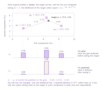
The one-dimensional case. Consider a simplified one-dimensional scenario where the predictions and the target are just points on a line as the figure below shows. Before the target arrives, the gate expresses a mild prior preference, distributing weights of , and across three experts. Once the target is revealed, we measure the gap between and each expert's prediction . Because Expert 2 () lands extremely close to the target, its likelihood increases. The posterior incorporates this evidence, sharpening the gate's guess that this specific case should be of responsibility of Expert 2 due to how close to the target this expert prediction was. The crucial takeaway is the difference between these two states,

which forms the exact gradient. The gate is heavily rewarded (+0.53) for the expert that was right, and penalized (-0.30, -0.23) for the two that were wrong.

Three expert predictions on a value axis at 2.1, 6.8 and 9.5, with the target at 7.0. Below, two rows of bars: the gate's prior at 0.30, 0.45 and 0.25, and the responsibilities at 0.00, 0.98 and 0.02. The difference between the rows is given as the gradient on the gate. — One case, drawn in one dimension so the predictions and the target are points on a line. The gate is trained on the gap between the prior and the posterior.

The vector case. When is a vector, the underlying arithmetic remains completely unchanged; only the geometric interpretation of the likelihood shifts. The simple gap on a number line becomes a spatial distance. To understand how this works, we can break down the variables:

: The multi-dimensional space where the target and predictions exist, with representing the number of dimensions.
: The covariance matrix () is set to the identity matrix (). This is a way of stating that we treat every dimension equally and assume no correlation between them.
: The likelihood function. Instead of measuring a simple scalar gap, it evaluates the probability based on spatial distance.
: The multi-dimensional prediction vector generated by expert .
: The Euclidean norm, representing the standard straight-line distance between the expert's prediction and the actual target.

Looking at the figure, the dashed lines represent the Euclidean distance between the expert predictions () and the target vector () in 2D space. Because Expert 2 sits much closer to the target (0.72) than the others, its likelihood spikes. This spatial proximity drives the posterior up to 0.98, overriding the gate's uncertain prior. The resulting gradient, , actively rewards the closest expert (+0.53) and penalizes the rest.

The same case drawn on a plane rather than a line. Three expert predictions sit at the coordinates 2.1 and 2.5, 6.6 and 4.6, and 9.5 and 3.0, with the target marked at 7.0 and 4.0 and dashed segments giving the distances 5.12, 0.72 and 2.69. Below, the same two rows of bars: the prior at 0.30, 0.45 and 0.25, and the responsibilities at 0.00, 0.98 and 0.02. — Widening the target changes what counts as close, and nothing else. The prior, the posterior and the gap between them are the same quantities, arrived at by measuring the distance in every component at once.

Log likelihood gradient

Before differentiating, we must define the likelihood of the entire training set under our mixture model, denoted as . Because the training cases are independent, the total likelihood is simply the product of the marginal probabilities across all cases and experts. Taking the log of this product retrieves a sum over cases and experts :

This is exactly the objective function we defined earlier, just with the sign flipped and summed over the dataset. Maximizing is identical to minimizing . When we differentiate this objective with respect to the gate's pre-softmax activations (let's call them ), the resulting gradient arriving at the -th output unit is:

Where

comes from, step by step

Let's work with a single case and drop the superscript , since the sum over cases just carries through at the end. This means, just to be clear, that we drop and look at a single term of it. We also rename the summation index from to , so that is free to mean the one expert we are differentiating with respect to:

Write for the likelihood of the target under expert , and for the marginal that sits inside the logarithm:

Step 1. Differentiate the logarithm. To find the gradient with respect to (the raw pre-activation score computed by the gate for expert ) we apply the chain rule. Because the expert likelihoods are completely independent of the gating network, they act as constants here. The raw score reaches the marginal only through the gates, and it reaches every one of them, because the softmax denominator is shared. That is why the sum below runs over all and not just over :

Step 2. Differentiate the softmax. Let the denominator be , meaning the gate's output is . To find the derivative, we apply the standard quotient rule:

Take the denominator first, because it behaves the same way whatever is. Differentiating the sum with respect to , every term where is a constant and drops to zero:

so , whatever happens to be.

The numerator is where we have the two cases. depends on only when happens to be , so

Feeding those two into the quotient rule gives the two cases:

First: for the target unit (), we have , meaning both the top and bottom of the fraction depend on :

Second: for any other unit () we have is independent of . Its derivative is , meaning the first term of the quotient rule vanishes:

Both are the same expression, written with the Kronecker delta , which is when and otherwise:

Step 3. Substitute and split the sum. Putting that back into step 1, the delta picks out the single term and the multiplies the whole sum:

Step 4. Recognise the marginal. The sum that is left is itself , so the second term collapses:

and in the second term the on top and the underneath are the same number, so they cancel and leave the gate on its own:

Step 5. Recognise Bayes. The first term is exactly the responsibility defined earlier, a prior times a likelihood over the marginal:

Substituting that back into step 4 closes the chain for a single case:

Restoring the case superscript and summing over the training set turns back into and gives the result stated above, .

It is worth seeing which step did the work. The in step 1 comes from differentiating the logarithm, and it is precisely the normalising constant that turns the raw quantity into a posterior in step 5. Had the logarithm been inside the sum rather than outside it, there would be no shared , no normalisation, and no posterior. The competition and the clean learning rule come from the same placement of the logarithm.

With the derivation complete, we can see that this is a clean learning rule. The gate trains to predict its own posterior, settling only when the prior and the posterior perfectly agree. The gradient arriving at the individual experts reveals the other half of the story. To understand this update, we differentiate the likelihood with respect to the expert's output prediction, denoted as . Factoring in as the constant variance of our Gaussian distribution, the gradient for the expert is:

The familiar error term is there, scaled by . An expert is corrected in proportion to how responsible it was. Typically only one expert has a large posterior on any case, so in practice only one expert learns each training case, and different experts end up learning different cases. The specialisation is not arranged. It falls out of the derivative.

Sparsity was never imposed

If we follow the learning dynamics to their fixed point, a clear pattern emerges. An expert that wins a case is trained on it and improves, raising its likelihood for that region of the input space. This increased likelihood raises its responsibility, which correspondingly raises the gate's prior. Consequently, after training, the gating network nearly always assigns a mixing proportion of one to a single expert per case.

Note that there's no enforcing of a sparse gate. There is no top- operation or penalty for spreading the probability mass. The gate therefore naturally sharpens because doing so maximizes the likelihood.

While this allows a partitioned model to significantly outperform a single dense network on heterogeneous tasks, it completely fails to reduce computational cost. To compute the objective , the forward pass requires the prediction for every expert , as every expert is evaluated inside the sum. The posterior requires them all over again.

The gate ends up nearly one-hot, but we still evaluate every expert anyway. Ultimately, this makes the mixture more expensive than the standard dense layer we started with. The specialization comes for free, but the computational savings do not. Translating this specialization into actual efficiency is the challenge of the next section.