03 · Mixture of Experts

Compute You Can Skip

If the gate is zero, the expert never runs.

The previous section showed us how to achieve a great deal of specialization for each expert, but that specialization comes at a huge computational cost. The mixture objective successfully produces a gate that is nearly one-hot, meaning that for any given input, a single expert is doing essentially all of the work. Yet, the standard formulation forces us to evaluate the entire ensemble anyway. We compute every possible path, only to multiply almost all of those outputs by a weight infinitesimally close to zero.

The fix is structural, if a gate value is zero, simply do not run the corresponding expert. Decoupling the math from the execution is the core of conditional computation. The rest of this page explores exactly how this routing is implemented, what it buys us, and what it ultimately costs.

Evaluate only the winners

The layer's shape remains the same as we defined before. For a token and experts,

What changes is the definition of . Instead of a softmax over all scores, we keep the largest and discard the rest before the softmax runs:

Two details in that definition matter more than they look.

The mask comes before the softmax, not after. Discarded scores are set to so and they contribute nothing to the denominator. The survivors renormalise among themselves and sum to one. Masking after the softmax would leave the surviving gates summing to less than one, and the layer's output would collapse whenever the router was uncertain.
Exactly terms of the sum are now zero. That is a statement about the arithmetic. It becomes a saving only because we then refuse to evaluate when , which is a change to the implementation that the definition happens to permit.

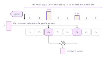
By enforcing this Top- mask, we fundamentally change how the token flows through the network, as shown in the figure below. When the token enters the layer, the router evaluates all eight available experts but enforces . As a result, six of the gate values are forced to zero, while the two winners renormalize to 0.65 and 0.35. Because we only evaluate an expert if this gate is non-zero, the token is physically routed to only and . The other six experts sit idle in memory. Their outputs are never computed, but the active predictions are weighted and summed to produce the final output. The parameters and the compute are no longer locked together.

A token enters a router that produces eight gate values. Two of them survive the top-2 and are shown as bars of 0.65 and 0.35; the other six are zero. A single line carries the token to only those two experts, the other six are outlined and unused, and the two active outputs are summed into the layer's output. — The parameters and the compute have come apart. All eight experts are stored and two are run, so the parameter count follows while the arithmetic per token follows . At and that is thirty two times the parameters of a dense block for the same arithmetic.

The arithmetic, again

Recall from The Layer That Reads Everything that a dense transformer block contains parameters and consumes FLOPs per token. In that paradigm, compute is strictly tied to capacity. However, when we apply conditional computation to total experts with the top active, the behavior changes. Let's start by highlighting the number of parameters and FLOPs per token:

Because memory scales with total experts () while arithmetic scales only with active experts (), nothing forces them to move together meaning that the parameter count and the compute cost are now two independent axes. As an example, consider the numbers from the dense layer, and , at experts and :

Quantity	Dense block	Sparse block, ,
Parameters	134,217,728 (~134 million)	8,589,934,592 (~8 billion)
FLOPs per token	268,435,456 (~268 million)	536,870,912 (~536 million)

While the sparse layer requires storing 64 times as many parameters, its operational cost only doubles relative to the dense block. To contextualize this efficiency, a dense block restricted to that same 536 million FLOP budget could only support 268 million parameters. The sparse architecture leverages these independent degrees of freedom to achieve a 32x increase in capacity without altering the arithmetic cost.

The line is broken

In The Layer That Reads Everything we drew every dense block on a single line through the origin, with parameters on one axis and cost per token on the other, and called the region underneath empty. Guess what, it is not empty any more!

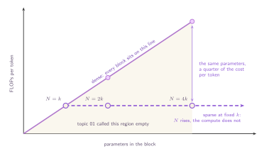
The same plane as for the dense layer, parameters against per-token FLOPs. The dense family lies on the diagonal. A dashed horizontal line of sparse models extends to the right at a fixed height, marked with the number of experts, showing that the parameter count grows while the cost per token stays constant. — Fix and raise , and the model moves right without moving up. The dense family could only travel along the diagonal.

The dense architecture has one direction available to it. The sparse one has two, and they are separately controllable: chooses how much arithmetic a token pays for, and chooses how much the layer is allowed to know.

What the trick costs

Nothing here is free, here are four major costs which are already visible.

The selection is not differentiable. is a step function of the scores. Gradient only flows through the experts that were chosen and the gate values that weighted them, and it does not reach the choice itself, or any expert that was not chosen.
The memory does not shrink. All experts must physically exist in memory. At , the layer rarely fits on a single device, meaning tokens must be transmitted over a network wherever their assigned expert resides, and the results routed back. Conditional compute inevitably causes communication overhead.
The assignment is ragged. The router dynamically decides how many tokens land on each expert at runtime. This directly clashes with hardware accelerators, which demand predictable, fixed-size matrices determined in advance.
The objective is no longer the one that specialised. The competition in Committee or Competition came from the log of a sum of per-expert likelihoods, which scores the experts separately. A sparse layer is trained on the task loss instead, with the outputs combined by a weighted sum, and that is the committee of that chapter. The selection is still hard, because makes it hard, but nothing in the loss now prefers a router that sends different tokens to different experts. The chapter on load balancing, Teaching the Router to Share, is where the field puts that pressure back by hand.

We kept the architecture that specialises and replaced the objective that made it specialise. The selection is still hard, because makes it hard, but nothing in the loss now prefers a router that sends different tokens to different experts, and nothing prevents one expert from taking everything. Later topics will go through this part in more detail.