InfoNCE Loss

Contrastive Predictive Coding

"In this paper we propose the following: first, we compress high-dimensional data into a much more compact latent embedding space in which conditional predictions are easier to model. Secondly, we use powerful autoregressive models in this latent space to make predictions many steps in the future. Finally, we rely on Noise-Contrastive Estimation for the loss function in similar ways that have been used for learning word embeddings in natural language models, allowing for the whole model to be trained end-to-end."

The overall goal of Oord et al. (2018) is to learn representations that encode the underlying shared information between different parts of a high-dimensional signal, while discarding low-level information and noise that is more local.

The problem with predicting in input space

One natural approach to self-supervised learning is to predict future observations directly in the raw input space. Given a context (for example, the past frames of a video), we could try to model the conditional distribution over future observations .

This runs into two difficulties:

1. Unimodal losses are not useful. Mean-squared error and cross-entropy penalise every pixel or token equally, regardless of whether the error is in a semantically meaningful feature or in irrelevant noise.
2. Generative models are expensive. Powerful conditional generative models can capture the full distribution, but they are computationally intensive and tend to waste capacity modelling local, low-level details of while ignoring the context .

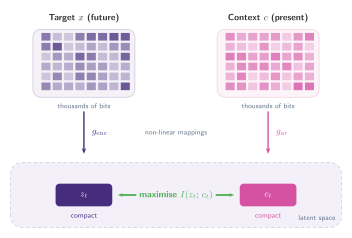
Consider images as a concrete example. A single image may contain thousands of bits of information, but the high-level latent variable we care about (say, the object category) requires only about 10 bits for 1,024 classes. Modelling directly forces the model to predict all those thousands of bits, most of which are irrelevant to the shared structure between and .

The CPC solution: encode, then maximise mutual information

Instead of predicting in the input space, CPC (Contrastive Predictive Coding) encodes both the target (future) and the context (present) into compact distributed vector representations via non-linear learned mappings. The encoder maps the target observation into a latent vector , while an autoregressive model summarises the context into .

The training objective is to maximally preserve the mutual information of the original signals and in this latent space. Mutual information between two random variables and is defined as

The ratio inside the logarithm, , measures how much knowing changes our belief about .

When is informative about , the conditional concentrates on the values of that are consistent with , making this ratio large. When tells us nothing, and the ratio equals one (contributing zero to the sum).

By maximising the mutual information between the encoded representations (which is bounded by the Mutual Information between the original input signals), the model learns to extract the underlying latent variables that and have in common, while discarding the details specific to each.

Formal Contrastive Predictive Coding

Let us now rewrite the intuition above in the paper's formal notation. A non-linear encoder maps each observation to a latent representation . An autoregressive model then summarises all latent vectors up to time into a single context vector .

As argued above, we do not predict future observations directly with a generative model . Instead we model a density ratio that preserves the mutual information between and :

• is the score function that measures how compatible a future observation is with the current context . The subscript indicates that we use a different scoring function for each time step into the future.
• is the conditional density of the future observation given the context. This is what a generative model would try to compute directly.
• is the marginal density of the future observation, regardless of context. Dividing by this term removes the "base rate" of , so that only reflects what tells us about .
• stands for "proportional to" (up to a multiplicative constant). The density ratio does not have to integrate to one, so can be unnormalised.

Although any positive real score function could be used, the paper chooses a simple log-bilinear model:

A separate linear transformation is used for each future step . Alternatively, non-linear networks or recurrent models could replace this bilinear form.

By modelling the density ratio and inferring with an encoder, we relieve the model from having to reconstruct the full high-dimensional distribution over . Although we cannot evaluate or directly, we can sample from these distributions, which allows us to use techniques such as Noise-Contrastive Estimation that are based on comparing the target value with randomly sampled negative values.

What this means in plain terms

Putting it all together, CPC works in three steps:

1. Compress. Given a sequence of observations (audio frames, image patches, text tokens), compress each one into a small vector , then build a summary of everything seen so far.
2. Score. The score function takes the context and a candidate future observation , and returns a number: high if is a plausible continuation, low if it is not. Because is proportional to the density ratio , a high score means is more likely given this context than it would be on average.
3. Discriminate. Given the context so far, can the model pick out what actually comes next from a set of random alternatives? The model never needs to reconstruct pixels or tokens; it only needs to tell real continuations apart from random ones.

InfoNCE Loss

We now have all the ingredients: an encoder that produces latent vectors , a context summary , and a score function that measures how compatible a candidate is with the context. The question is: how do we turn this into a training objective?

The idea is simple. Given a context , we draw one positive sample (the true future observation) and negative samples drawn randomly from the data. We then ask the model to identify the positive among all candidates. This is a classification task.

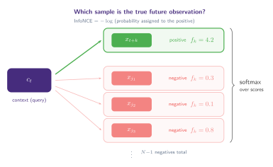
The loss for a single prediction is the negative log-probability that the softmax assigns to the positive sample:

Substituting the log-bilinear form , this becomes:

Reading the equation

Let us unpack this piece by piece:

• Numerator : the score assigned to the positive sample. The dot product measures how well the true future aligns with the context. We want this to be large.

• Denominator: the sum of scores over all candidates (one positive + negatives). This acts as a partition function, normalising the scores into a valid probability distribution via softmax.

• The ratio is therefore the probability the model assigns to the correct positive:

• The converts this probability into a cross-entropy loss. When the model is confident and correct, and . When it fails, and .

Temperature

In practice, a temperature hyperparameter is added to control the sharpness of the softmax distribution. The loss becomes:

• (sharp): The distribution becomes nearly one-hot. The model must be very confident. Hard negatives (those with high similarity to the context) dominate the gradient.
• (uniform): All candidates contribute equally. The loss becomes less discriminative and the learning signal is weak.
• Typical values: . SimCLR uses ; MoCo uses .

Gradient Analysis

Let denote the scaled score for candidate , and let be the probability the model assigns to candidate . The gradient of with respect to the context is:

The gradient pushes towards the positive representation and away from the probability-weighted average of all candidates. Hard negatives (those with high ) dominate the repulsion, so the model learns most from its mistakes.

For a negative sample :

Only negatives that the model confuses with the positive (high ) receive a meaningful gradient signal.

Connection to Mutual Information

The name "InfoNCE" comes from Noise-Contrastive Estimation applied to mutual information. The key theoretical result from Oord et al. (2018) is:

Minimising InfoNCE maximises a lower bound on the mutual information between the target and context. The bound is capped at , where is the total number of candidates (one positive + negatives). This motivates using large batch sizes: more negatives raise the ceiling on how much mutual information the loss can capture.

As the bound becomes tight and the estimator recovers the true mutual information.

InfoNCE in PyTorch

A minimal implementation of InfoNCE following the CPC framework. We simulate a sequence of observations, encode them, build context vectors with a GRU, and train using the InfoNCE loss to predict future latent representations.

# infonce_example.py
import torch
import torch.nn as nn
import torch.nn.functional as F
import torch.optim as optim

# ── Synthetic data: random sequences ────────────────────────────

def sample_sequences(batch_size=32, seq_len=16, input_dim=40):
    """Generate random sequences (e.g. audio frames, image patches)."""
    return torch.randn(batch_size, seq_len, input_dim)

# ── CPC model ───────────────────────────────────────────────────

class CPCModel(nn.Module):
    def __init__(self, input_dim=40, z_dim=64, c_dim=128, pred_steps=4):
        super().__init__()
        self.pred_steps = pred_steps

        # g_enc: non-linear encoder x_t -> z_t
        self.encoder = nn.Sequential(
            nn.Linear(input_dim, 128),
            nn.ReLU(),
            nn.Linear(128, z_dim),
        )

        # g_ar: autoregressive model z_{<=t} -> c_t
        self.autoregressive = nn.GRU(z_dim, c_dim, batch_first=True)

        # W_k: one linear prediction head per future step
        self.predictors = nn.ModuleList(
            [nn.Linear(c_dim, z_dim, bias=False) for _ in range(pred_steps)]
        )

    def forward(self, x):
        # Encode all observations: (batch, seq_len, z_dim)
        z = self.encoder(x)

        # Autoregressive context: (batch, seq_len, c_dim)
        c, _ = self.autoregressive(z)

        return z, c

# ── InfoNCE loss ─────────────────────────────────────────────────

def infonce_loss(z, c, predictors, pred_steps, n_negatives=16, tau=0.07):
    """
    z: (batch, seq_len, z_dim) — encoded observations
    c: (batch, seq_len, c_dim) — context vectors
    """
    batch_size, seq_len, z_dim = z.shape
    losses = []

    for k in range(1, pred_steps + 1):
        # Maximum timestep from which we can predict k steps ahead
        t_max = seq_len - k

        # Context at time t: (batch, t_max, c_dim)
        c_t = c[:, :t_max, :]

        # Positive: true future z_{t+k} for each t: (batch, t_max, z_dim)
        z_pos = z[:, k : k + t_max, :]

        # W_k * c_t: predicted future representation: (batch, t_max, z_dim)
        pred = predictors[k - 1](c_t)

        # Score positives: z_{t+k}^T W_k c_t / tau → (batch, t_max, 1)
        pos_scores = (pred * z_pos).sum(dim=-1, keepdim=True) / tau

        # Sample random negatives from other positions in the batch
        neg_idx = torch.randint(
            0, batch_size * seq_len, (batch_size, t_max, n_negatives)
        )
        z_flat = z.reshape(-1, z_dim)
        z_neg = z_flat[neg_idx]  # (batch, t_max, n_negatives, z_dim)

        # Score negatives: z_j^T W_k c_t / tau → (batch, t_max, n_negatives)
        neg_scores = torch.einsum("btd,btnd->btn", pred, z_neg) / tau

        # Concatenate: positive first, then negatives
        # → (batch, t_max, 1 + n_negatives)
        logits = torch.cat([pos_scores, neg_scores], dim=-1)

        # Label = 0: the positive is always at index 0
        labels = torch.zeros(batch_size, t_max, dtype=torch.long)

        # InfoNCE = cross-entropy over the candidates
        loss_k = F.cross_entropy(
            logits.reshape(-1, logits.size(-1)), labels.reshape(-1)
        )
        losses.append(loss_k)

    return torch.stack(losses).mean()

# ── Training loop ────────────────────────────────────────────────

model = CPCModel()
optimizer = optim.Adam(model.parameters(), lr=3e-4)

for step in range(3000):
    x = sample_sequences()

    z, c = model(x)
    loss = infonce_loss(z, c, model.predictors, model.pred_steps)

    optimizer.zero_grad()
    loss.backward()
    optimizer.step()

    if (step + 1) % 500 == 0:
        print(f"Step {step + 1:4d} | loss = {loss.item():.4f}")

# Expected output: loss ≈ 2.83 = ln(17)
# With random data there is no temporal structure to learn,
# so the model cannot do better than chance: 1/17 ≈ 5.9%

A few things to notice:

• We compute pos_scores and neg_scores separately, then concatenate them with the positive first. Since the positive is always at index 0, the label is simply 0 and the loss reduces to F.cross_entropy.
• Each prediction step has its own linear head predictors[k-1], corresponding to in the paper. This computes , the predicted future representation.
• Negatives are sampled randomly from all encoded observations in the batch. Each query gets n_negatives random candidates, scored via einsum.
• The temperature tau=0.07 sharpens the softmax. Both positive and negative scores are divided by before the cross-entropy.

Four things to keep from InfoNCE

1. InfoNCE is a softmax cross-entropy over similarity scores: classify the true future observation among random negatives.
2. Temperature controls the sharpness of the distribution and which negatives matter most.
3. The gradient is dominated by hard negatives, meaning samples the model currently confuses with the positive.
4. Minimising InfoNCE maximises a lower bound on mutual information , bounded by .