The previous section left accuracy with a number that reports partly on the model and partly on the crowd, and no way to separate the two. Balanced accuracy is the standard response, and it is a real improvement.
It is worth being precise about what it improves, because it is not what the name suggests. The prevalence commitment is not removed. It is replaced, and a cost commitment arrives in its place.
One substitution
Balanced accuracy is the mean of the two rates from section 02.
where is the share of positive cases the model catches at threshold , and is the share of negative cases it correctly leaves alone. Sensitivity and specificity, averaged.
Set that beside the identity section 02 established, which splits accuracy into the same two rates.
The two expressions have the same shape and differ only in their weights. Accuracy weights each rate by the share of the population its class occupies. Balanced accuracy weights them equally, which is to say it sets .
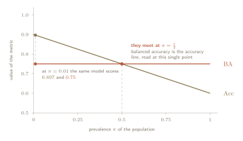
Balanced accuracy is not a correction applied to accuracy. It is accuracy, read at a prevalence of one half. Whatever population the test set was drawn from, the number reported is the accuracy this model would have achieved on a population holding equal numbers of the two classes.
One model throughout, with and . Its two rates never move, so is flat. slides from to because it reweights those same two rates by whoever is in the room. The two agree at exactly one point, and that point is .
What it genuinely fixes
Section 03 left accuracy with a scale that collapses. At a model that answers negative to everything already scores , and every model worth discussing is packed into the remaining hundredth.
That failure is gone entirely. Take any model that ignores its input. Answer negative always, and with , so . Answer positive always, and with , so . Both score exactly one half, at every prevalence, with no exceptions. Chance is pinned to and stays there, so the entire range of the metric is available to describe the model.
The invariance is real too, for the reason section 02 gave. Balanced accuracy is assembled from and , and both divide by a column total, so recruiting more negatives changes neither. On the first of the three failures, dependence, balanced accuracy is a strict improvement over accuracy.
The same condition section 02 attached still applies. The claim concerns a change in how many, not a change in who. Negatives drawn from a different population move , and balanced accuracy moves with it.
The cost that arrives instead
Section 03 made accuracy legible by putting its payoff table on the page. Balanced accuracy has one too.
where is the prevalence of the evaluation set (Flores et al., 2025). The entries are no longer and . Each correct call is now worth the reciprocal of twice its own class's share, so the rarer a class is, the more a correct call on it pays.
The entries are payoffs in an arbitrary unit, and only their ratio carries any meaning. At the table assigns payoff units to a caught positive and to a negative correctly left alone. Dividing one by the other cancels the unit, and in general
which is for . Balanced accuracy declares one caught positive worth ninety-nine negatives correctly left alone, or equivalently one missed positive worth ninety-nine false alarms. For some problems that is a defensible exchange rate. But it is not neutral, and most importantly it wasn't actually chosen. Meaning it was fixed by the base rate of whichever evaluation set happened to be used.
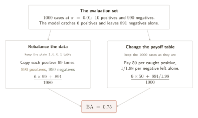
The same number can be reached from either direction, and Flores et al. write it both ways. A small example shows why. Take cases at , so positives and negatives. At some threshold the model catches of the positives and correctly leaves of the negatives alone, which makes ordinary accuracy .
Both routes reuse the same five counts.
is the number of cases, and the two class counts. So and .
Route one: rebalance the data, keep the table. Copy each positive times, then count correct answers as usual.
Route two: keep the data, change the table. Pay each case the entry the table above gives it.
The same , twice, and neither route is the that accuracy reported. The first describes a population that does not exist. The second describes the implicit cost structure. They are the same arithmetic.
The two routes drawn side by side. Reweight the data and keep the plain payoff table, or keep the data and reweight the table. The arithmetic meets at , and neither branch passes through the that ordinary accuracy reports on the same cases.
Where the threshold lands
Section 03 showed that for a calibrated score, accuracy is maximised by predicting positive when . That one half came out of a symmetric payoff table where both correct answers were worth the same, so the tie sat in the middle. The table above is not symmetric, so the tie sits somewhere else. Take a single case whose posterior is , and price the two things we could do with it. Both prices come straight from the table.
Flag it. With probability the case really is positive and the table pays . With probability it is negative and the table pays .
Leave it. With probability the case really is negative and the table pays . With probability it is positive and the table pays .
Flagging is worth it when the first beats the second, which we can write and thus yields:
The term sits on both sides and cancels, which is why the answer comes out as clean as it does.
Let's read the statement above step by step. When the two options are worth exactly the same and the metric is indifferent. Above it, flagging pays. Below it, leaving pays. The threshold that maximises balanced accuracy is therefore the prevalence itself:
One caveat on that last step. The rule was derived for the posterior , and it becomes a rule about the score only when the score is the posterior, which is to say when the model is calibrated. For an uncalibrated score the optimum still exists, but it has to be found by sweeping rather than read off.
Balanced accuracy is maximised by thresholding the posterior at the prevalence itself. At that instructs us to act on every case whose probability exceeds one percent. For a cancer screening programme this may well be correct. For a spam filter it would quarantine most of the inbox. Both rules come out of the same metric, and the metric chose between them by reading the base rate off the data rather than by asking anybody what a mistake was worth.
A different assumption, not the absence of one
What balanced accuracy estimates is perfectly well defined: the accuracy this model would achieve on a population containing equal numbers of the two classes. The question is whether that population is one anybody will meet.
Two settings where it is the right quantity:
comparing one model across several datasets whose class mixes differ for reasons of collection rather than deployment,
benchmark reporting where no deployment population is being claimed at all.
And one where it is not. Wherever somebody will act on the model at a known base rate, one half is simply the wrong prevalence, and the observed was the better guess of the two. Replacing a measured quantity with a fixed one is only a repair if the fixed one is closer to the truth.
Balanced accuracy stays inside the columns. It is built from and , and inherits both their invariance and their silence about cost. The next section takes up the first metric that leaves the columns.