learning-ai.cafe learning-ai.cafe / Metrics / 05

05 · Metrics

Precision

A point on the ROC curve, read at a declared prevalence.

Section 02 sorted the confusion matrix into columns and rows, and left precision on the wrong side of that division. Every metric so far has divided by a column total, which is a class count. Precision divides by a row total, which is a decision count, and a row holds cases from both classes. This section works out what that costs.

A row, not a column

Precision, also called the positive predictive value (PPV), is the share of flagged cases that really were positive.

The conditioning bar has moved. Section 02 conditioned on the truth and asked what the model did. Precision conditions on what the model did and asks about the truth. It runs the same question backwards, which is why it needs something the two rates did not.

Write the two cells in terms of the rates. Of the positive cases, a share clear the threshold. Of the negative cases, a share do.

Substitute, then divide through by .

This is the identity the whole section rests on (Richardson et al., 2024). Writing puts it in the tutorial's notation.

which is Bayes' theorem, and it is worth naming as such. and are likelihoods, the two ways a case can end up above the threshold. is the prior. Precision is the posterior, the probability that a flagged case is genuinely positive. Later sections return to this, because a posterior is exactly the object calibration is about.

The third input

Read the identity as a recipe and count what goes into it. Two of the three inputs, and , come from the model at a chosen threshold. The third, , comes from the world.

Take one operating point and hold it still: a classifier that catches of the positives while wrongly flagging of the negatives (Richardson et al., 2024). Nothing about it will change below. Changing only the prevalence yields:

Same model, same threshold, same scores on every case. The precision more than halves. Precision is not a property of the classifier. It is a property of the classifier and the population, fused into one number with no way to separate them.
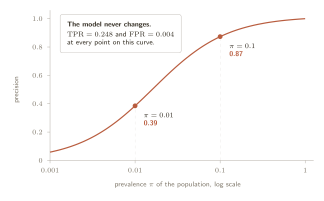
Precision plotted against prevalence on a logarithmic axis running from 0.001 to 1, for a single fixed operating point with TPR 0.248 and FPR 0.004. The curve rises from near zero at the far left to almost one at the right, passing through 0.39 at prevalence 0.01 and 0.87 at prevalence 0.1, both marked with dots. A box states that the model never changes across the whole curve.

One operating point, every prevalence. The model's two rates are fixed at and across the whole curve, so every bit of the movement belongs to . Note the direction: the rarer the positive class, the lower the precision.

The negative side of the table behaves the same way. The share of cases the model let through that really were negative is the negative predictive value, it divides by the other row, and it moves with for the same reason and in the opposite direction.

Which way it leans

Precision is often reached for as the answer to accuracy's problem under imbalance. It is worth putting the two side by side as falls, because they do not fail in the same direction.

  • Accuracy rises toward , since the negatives take over the average and the model handles them well.
  • Precision falls toward zero, since the flagged row fills with false positives drawn from an ever larger negative class.
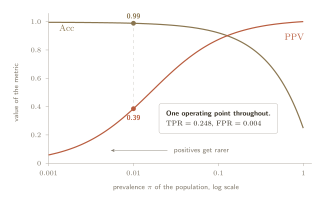
Accuracy and precision plotted together against prevalence on a logarithmic axis from 0.001 to 1, for a single fixed operating point. The accuracy curve starts near one at the far left and falls steeply toward the right. The precision curve starts near zero at the far left and rises toward one. They slope in opposite directions and cross near prevalence 0.13. A dashed line at prevalence 0.01 marks accuracy at 0.99 and precision at 0.39. An arrow points left, labelled positives get rarer.

The same operating point as before, graded two ways. Read the plot right to left, in the direction the arrow points, and the positives get rarer: climbs while collapses. At the two verdicts on one unchanged model are and , a disagreement of .

Both are reporting the crowd. One flatters the model as the positives get rarer and the other punishes it, and neither is measuring something the model did. Swapping accuracy for precision does not remove the prevalence commitment. It reverses the sign of the error.

There is a second, quieter problem at the same end of the scale. Push high enough and the model flags very few cases, so the denominator is built from a handful of them. The estimate becomes extremely noisy, and at the limit where nothing is flagged, precision is undefined rather than zero. That is the second of the three failures, variance rather than dependence, and a later section takes it up properly.

When precision is the right number

None of the above makes precision a bad metric. It makes it a conditional one, and there is a question it answers better than anything else in this tutorial: this alert just fired, how much should I believe it?

That is the question the person on the receiving end actually asks, so precision is exactly the right object. For example radiologists reading flagged scans and analysts working a fraud queue. Sensitivity and specificity cannot answer it, because they condition on a truth nobody knows yet.

The condition is that the in the identity has to be the prevalence of the population the alert came from. So precision is correct when a deployment prevalence has been declared, and the rule that follows is simple: report precision with the prevalence it assumes, or do not report it.

Where it goes wrong

Two failures follow directly, and both are common.

  1. Comparing across populations. Two models evaluated on datasets with different base rates cannot be ranked by precision, because the comparison contains a term neither model is responsible for. The same holds for one model in two clinics.
  2. Inheriting a prevalence nobody chose. Test sets are often built by case-control sampling, or by keeping all the positives and subsampling the negatives. The resulting is an artefact of collection. Precision computed on it is a real number about a population that was assembled for convenience.

Both have the same repair, and it is the one the identity suggests. and survive the move between populations, so carry those, and recompute precision at whichever prevalence is being claimed.

learning-ai.cafe

Metrics

Leaving out parts of the truth: an analysis of metric estimation, theoretical assumptions, and points of structural failure in ML/DL.

  1. 01 What a Metric Actually Is
  2. 02 TPR and FPR
  3. 03 Accuracy
  4. 04 Balanced Accuracy
  5. 05 Precision
    1. A row, not a column
    2. The third input
    3. Which way it leans
    4. When precision is the right number
  6. 06 F1
  7. 07 ROC and AUROC
  8. 08 Partial AUROC
  9. 09 PR Curves and AUPRC
  10. 10 Variance at Low Prevalence
  11. 11 Calibration and ECE
  12. 12 Brier Score
  13. 13 Log Score
  14. 14 Net Benefit
  15. 15 Bounded DCA Log Score
  16. 16 What to Report
  17. 17 References

Who built this page

Every merged contribution is typed and scored at review. Chips next to a heading show who touched that section. Scores feed the contributor share of project support.

History

    Propose a change

    Settings

    Language
    Appearance
    Accent
    Font
    Text size
    Column width
    Book